Credible and Confidence Intervals
Credible Interval (or Region)
A Credible Interval or region (for multi-dimensional cases) for parameter \(x\) consists of a lower estimate \(L\), and an upper estimate \(U\), such that the probability of the true value being within the interval estimate is equal to \(\alpha\). For example, a 95% credible interval (i.e. \(\alpha = 0.95\)) for a parameter \(x\) is given by \([L, U]\) such that
The smaller the test size, the wider the confidence interval will be, and the greater \(\alpha\), the smaller the confidence interval will be. The evaluation of credible intervals follows a bayesian approach, where one assumes a prior probability density function that models the likelihood of the parameter, given its possible range. Once the prior function is established, the Bayes theorem is used to devise the posterior distribution of the parameter given its current estimate, and to calculate the credible interval.
Background
In binary classification problems where each sample is i.i.d. (independent and identically distributed random variables), success/failure tests are binomially distributed (that is, composed of a number \(n\) of Bernoulli trials using a biased coin with “unknown” proportion \(p\)):
where:
\(n\) is the total number of trials for a particular experiment,
\(k\) is the number of successes within those trials, and
\(p\) is the true probabibility, which is unknown, and that we are trying to estimate from experiments.
To estimate \(p\), the true value for the unknow probability, given \(k\), the number of successes observed in a concrete experiment, we apply the Bayes theorem:
The value of \(P(k)\) does not depend on \(n\) and can be recast as a marginalized version of \(P(k\mid p)\), which will help us later:
In the case of a binomial distribution, \(P(k\mid p)\) is known (first equation). \(P(p)\) is normally called the prior probability density, and corresponds to a known (or most likely) density distribution for the parameter \(p\). The choice of this prior will of course affect the overall aspect of the posterior distribution \(P(p\mid k)\) we are trying to estimate.
A typical choice for this prior is a Beta distribution. As it turns out, a Beta prior will generate a (conjugate) Beta posterior:
This formulation provides us with a complete representation for the posterior of \(p\), allowing the calculation of credible intervals, via integration. The values \(\alpha\) and \(\beta\) are hyper-parameters which control the skewness of the Beta distribution towards the maximum or the minimum respectively. As there is no reason to favour one more than the other, these are typically set to matching values \(\alpha=\beta=\lambda\).
Two classical settings are often used:
\(\lambda = 1\) (a.k.a. a “flat” prior)
\(\lambda = 0.5\) (a.k.a. Jeffrey’s prior)
In practice, changing \(\lambda\) does not affect much the credible
interval calculation. To calculate the credible interval for a binary variable
using a flat or Jeffrey’s prior, use
credible.bayesian.utils.beta(), providing
\(k\), \(l=(n-k)\), \(\lambda\) and how much coverage you would
like to have (typically 0.95 - 95%).
Applicability to Figures of Merit in Classification
[GOUTTE-2005] extended this analysis to classifical figures of merit in classification, with a similar reasoning as used for accuracy on the previous section:
Precision or Positive-Predictive Value (PPV): \(p = TP/(TP+FP)\), so \(k=TP\), \(l=FP\)
Recall, Sensitivity, or True Positive Rate: \(r = TP/(TP+FN)\), so \(k=TP\), \(l=FN\)
Specificity or True Negative Rage: \(s = TN/(TN+FP)\), so \(k=TN\), \(l=FP\)
Accuracy: \(acc = TP+TN/(TP+TN+FP+FN)\), so \(k=TP+TN\), \(l=FP+FN\)
Jaccard Index: \(j = TP/(TP+FP+FN)\), so \(k=TP\), \(l=FP+FN\)
Functions at credible.bayesian.metrics can calculate the above
quantites in a single shot from counts of true and false, positives and
negatives, the \(\lambda\) parameter, and the desired coverage.
Note
For comparing two systems according to their F1-score, please see Comparing 2 systems.
Confidence Interval
A confidence interval corresponds to a frequentist approach to the estimation of a range of values for an unknown parameter \(p\). More formally, a 95% confidence interval means that if the same sampling procedure were repeated n times from the same population, approximately 95% of the estimated intervals would include the true value of the parameter. Whereas in the Bayesian approach the interval is fixed and the parameter \(p\) is subject to random process, in the frequentist approach, the parameter \(p\) is fixed and the interval is subject to randomness.
Note
Common misconception
A 95% confidence interval does not mean that there is a 95% probability that the true parameter lies inside the computed interval.
The confidence level instead describes the long-run reliability of the estimation procedure: over many repeated experiments, approximately 95% of the constructed intervals would contain the true population parameter.
There are several proposed ways to calculate a confidence interval, the correct choice depends on the data being analyzed. This package implements two categories:
The first category contains methods specifically designed for binomial proportions. These methods assume that the quantity of interest can be modeled as the proportion of successes observed over a fixed number of independent Bernoulli trials. Under these assumptions, the goal is to estimate the unknown success probability \(p\) from the number of observed successes and failures. This package implements several methods that differ by the “conservativeness”, or how large the interval will be for the same coverage. Except for specific method parameterization (\(\lambda\)), they should (almost) work as a drop-in replacement for
credible.bayesian.utils.beta():Wilson, 1927, [WILSON-1927]:
credible.frequentist.utils.wilson()Clopper-Pearson, 1934, [CLOPPER-1934]:
credible.frequentist.utils.clopper_pearson()Agresti-Coull, 1998, [AGRESTI-1998]:
credible.frequentist.utils.agresti_coull()
The second category implements non-parametric bootstrap confidence intervals.
Non-parametric bootstrap, [EFRON-1994]:
credible.frequentist.utils.bootstrap_metric()
Unlike the methods above, bootstrap intervals are not restricted to binomial proportions and can instead be applied to more general scalar metrics computed from labels and predictions or scores. Non-parametric bootstrapping estimates uncertainty by repeatedly resampling the observed dataset with replacement and recomputing the target metric on each resampled dataset. The resulting empirical distribution of the metric is then used to derive confidence intervals, typically from percentile quantiles (e.g., 2.5th-97.5th percentiles for a 95% CI).
Important
non-parametric does not mean assumption-free
Although bootstrap methods are distribution-free in the sense that they do not assume a specific parametric form (e.g., Gaussian or binomial), they are not assumption-free. They rely on the assumption that the observed sample is representative of the population and that observations are independent and identically distributed (IID).
Recommended usage through the metrics API
Because this package supports both Bayesian credible intervals and frequentist confidence intervals,
credible exposes a common metrics interface at credible.metrics. In most cases, users can
call the same metric function and select the uncertainty-estimation procedure through the method argument.
Setting method="bayesian" computes Bayesian credible intervals, while setting method="frequentist"
computes bootstrap confidence intervals.
To use this interface, simply call a metric function and pass the desired method along with any relevant
arguments. For example:
import numpy
from credible.metrics import accuracy_score

rng = numpy.random.default_rng(42)

nb_samples = 50

y_true = numpy.ones(nb_samples, dtype=bool)
y_true[:10] = 0

# y_pred has exactly 5 errors, therefore accuracy is 90%
y_pred = y_true.copy()
y_pred[:5] = numpy.logical_not(y_pred[:5])

value, mode, lower, upper = accuracy_score(
    y_true,
    y_pred,
    coverage=0.95,
    method="bayesian",
    lambda_=1.0,
)

print(f"Bayesian accuracy: {value:.3f} [{lower:.3f}, {upper:.3f}]")

value, mode, lower, upper = accuracy_score(
    y_true,
    y_pred,
    coverage=0.95,
    method="frequentist",
    n_bootstraps=1000,
    rng=rng,
)

print(f"Bootstrap accuracy: {value:.3f} [{lower:.3f}, {upper:.3f}]")
Bayesian accuracy: 0.900 [...]
Bootstrap accuracy: 0.900 [...]
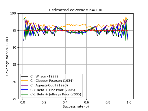
Conservativeness
When talking about credible or confidence intervals, one the most important aspect relates to the method conservativeness. A method that is too conservative (pessimistic) will tend to provide larger than required intervals that surpass the required coveraged. If you are using this to compare systems (e.g. compare models A and B performance through the same database), then a too-pessimistic approach may result in overlapping performance intervals for both systems. Therefore, it is preferrable to use a technique that is as precise as possible.
Estimating conservativeness is a difficult task. The main problem relates to
the underlying hypothesis samples are issued from a binomial distribution
(i.e., are true Bernoulli trials). Considering that to be true, you can test
the various methods coverage regions through simulation. The function
credible.curves.estimated_ci_coverage() can help
you with that task, and provides an usage example for the various intervals
implemented in this package:
(Source code, png, hires.png, pdf)
Comparing 2 systems
According to [GOUTTE-2005], 2 distinct systems may be compared by considering either two specific use-cases: if both systems are exposed to the same (paired comparison) or different data (unpaired). As a rule of thumb, paired tests carry stronger constraints and therefore have the potential provide more sensitive credible intervals.
Unpaired comparison
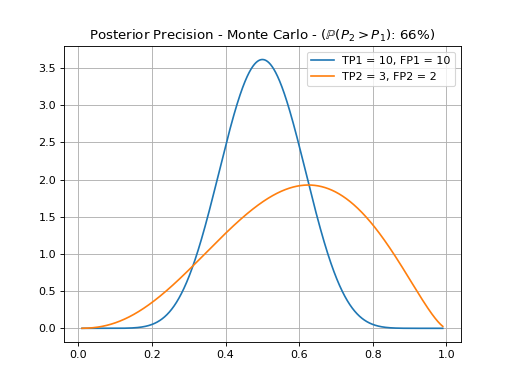
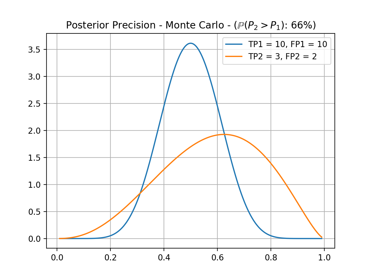
To perform an unpaired comparison of two systems, we first assume each system have a fixed threshold and therefore can produce two sets of true and false positive and negative scores. Under these conditions, one may compare two figures of merit (Applicability to Figures of Merit in Classification), taken as base their posterior beta distributions. This cannot be done analytically, so we resort to a Monte Carlo simulation. In the following example, we compare the precision and recall of two systems previously tuned.
(Source code, png, hires.png, pdf)

From this, we can assert that system’s 2 precision is only 65% (empirically) likely to be better than system’s 1 precision. A test for a 95% credible interval, in this case, would fail. Of course, we can apply the same reasoning for the recall.
(Source code, png, hires.png, pdf)
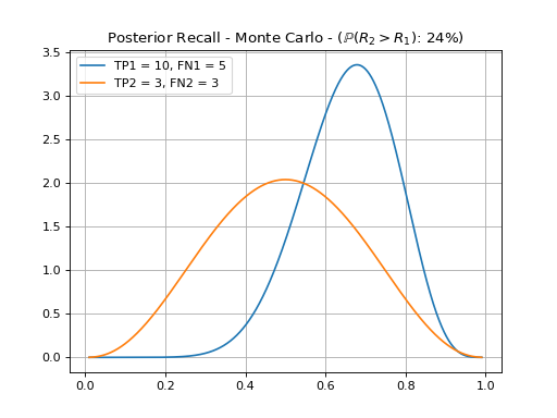
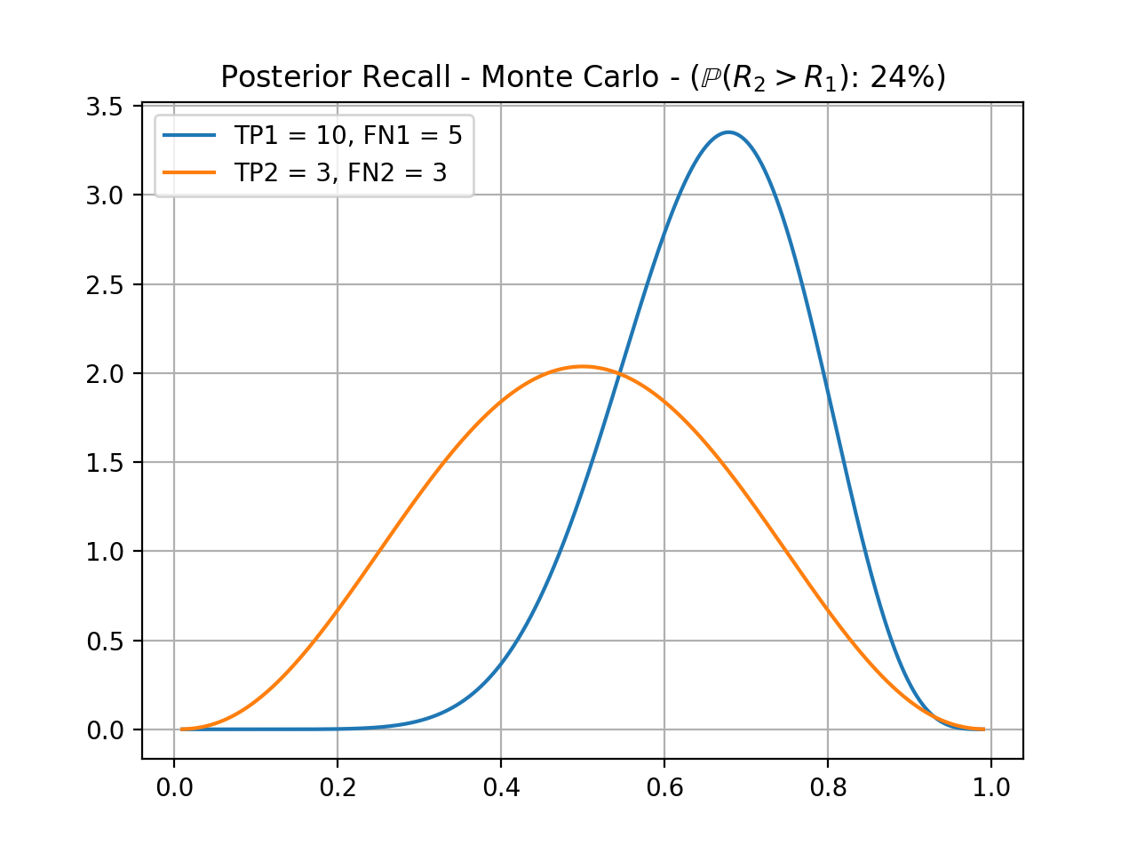

Here, we see that there is only a 24% probability that system’s 2 recall is better than system 1. Again, a check for a 95% margin would fail.
Comparing F1-Scores
Comparing F1-scores cannot be done with the procedure above, using a Beta posterior, according to [GOUTTE-2005]. We resort again to Monte Carlo simulations for this.
(Source code, png, hires.png, pdf)
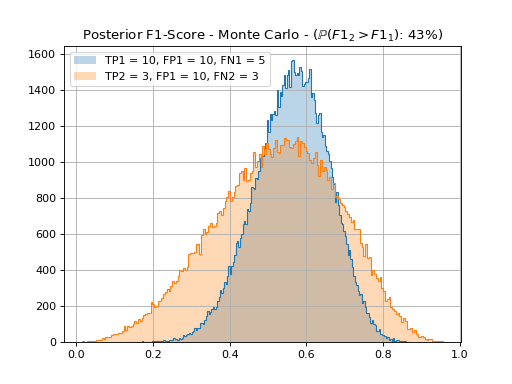
From this, we cannot assert that neither system’s 1 or 2 F1-score is greater than the other one with a 95% confidence.
ROC and Precision Recall Curves
It is often useful to explore multiple thresholds at the same time, instead of tuning each system to a set of thresholds. This package allows you to plot ROC and Precision-Recall curves including credible/confidence interval bounds. We simply repeat the procedure above for each threshold and plot the results. The bounds of the curve are calculated taking into consideration the credible interval at that particular point, in all four directions. The calculation of the upper bound for a typical performance curve is examplified below:


The lower bounds of a performance curve are calculated using the same principle, using the lower ellypse formed by the lower bounds of the credible interval.
Here is an example on how to use the built-in procedures for plotting ROC curves:
(Source code, png, hires.png, pdf)
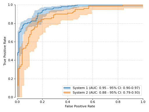
The plotting procedure produces the area under the ROC curve (AUROC) for all three curves: the normal ROC, as well as the lower and upper bounds, which allows for the estimation of the 95% credible interval of that measure. In this example, it is possible to observe both system performances overlap a bit, from the perspective of the AUROC. A more thorough analysis would require the selection of a threshold for each system, and a more detailed CI analysis.
We can also create Precision vs. Recall plots. Here is the above system from that perspective.
(Source code, png, hires.png, pdf)
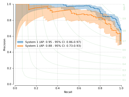
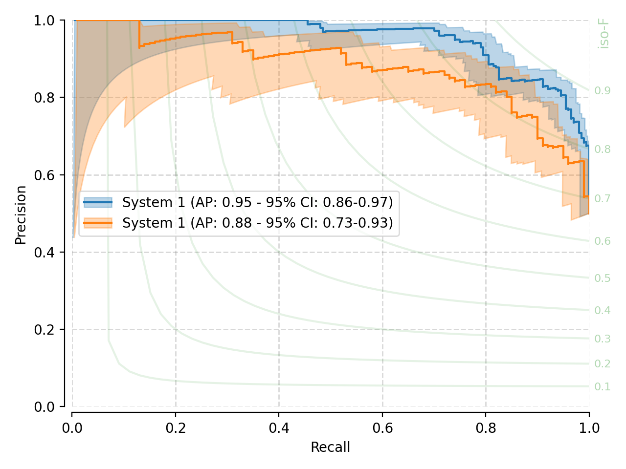

With the precision-recall curves, our stock canvas also includes iso-F1 lines, which show equal-valued F1-score segments. Also on this view, both systems present significant overlap in terms of the area under the PR curve (AUPRC).
Paired comparison
Bayesian approach
The paired (binary) comparison described in [GOUTTE-2005], equations 16 and 19 is implemented. It is an extension of the bayesian approach described for the various figures of merit (precision, recall, specificity, etc), by considering a Dirichlet posterior (generalization of the beta posterior for a multinomial distribution), with the following parameters:
\(N_1\): then number of times system 1 gets the output right (matches label), and system 2 gets it wrong
\(N_2\): then number of times system 2 gets the output right (matches label), and system 1 gets it wrong
\(N_3\): then number of times system 1 and 2 outputs match, even if they do not match the reference label
Note
In a paired comparison, both systems to be compared (systems 1 and 2) have been previously tunned, and output only binary outcomes. The binary outcomes of each system are compared with the reference labels to determine correct or incorrect hypotheses.
Notice \(N = \sum_i N_i\) corresponds to the total number of samples available for the comparison. By consequence, \(\pi_i = N_i / N\) corresponds to the multinomial probability one of the above outcomes take place. The implemented posterior has the following form:
Each alpha_k corresponds to the prior information about the distribution of each probability. Typically, a symmetrical prior is used such as Jeoffrey’s (\(\alpha_k=0.5\)) or flat (\(\alpha_k=1\)). Given the various relationships above, the implemented function inputs only \(N_k\) and \(\alpha_k\). The outcome is computed via Monte-Carlo simulation, for which you must decide on the number of samples. Values in the order of millions are typically used for a more precise estimation.
The following piece of code simulates two systems and runs a paired comparison
using the built-in function
credible.bayesian.utils.compare_systems():
print(f"Total number of samples: {nb_samples}")
print(f"Ratio negatives/positives: {100*ratio:.0f}%")
print(f"System 1 accuracy: {100*system1_acc:.2f}%")
print(f"System 2 accuracy: {100*system2_acc:.2f}%")

# calculate when systems agree and disagree
n1 = numpy.count_nonzero(
    (~numpy.logical_xor(system1_output, labels))  # correct for system 1
    & numpy.logical_xor(system2_output, labels)   # incorrect for system 2
)
n2 = numpy.count_nonzero(
    (~numpy.logical_xor(system2_output, labels))  # correct for system 2
    & numpy.logical_xor(system1_output, labels)   # incorrect for system 1
)
n3 = nb_samples - n1 - n2
print(f"N1: {n1}; N2: {n2}; N3: {n3}")
# N.B.: rng = numpy.random.default_rng(1234) # was initialized earlier
prob = compare_systems([n1, n2, n3], [0.25, 0.25, 0.25], 1000000, rng)
print(f"Prob(System1 > System2) = {100*prob:.2f}%")
Total number of samples: 50
Ratio negatives/positives: 20%
System 1 accuracy: 90.00%
System 2 accuracy: 84.00%
N1: 8; N2: 5; N3: 37
Prob(System1 > System2) = 80.10%
Frequentist approach
In the frequentist setting, a permutation test provides a natural alternative for paired system comparisons.
The test starts from the null hypothesis that the two systems have equal performance on the evaluated samples.
Under this null hypothesis, the outputs of the two systems are exchangeable within each paired sample.
The null distribution is therefore obtained by randomly swapping the two system outputs within each sample
and recomputing the performance difference. This procedure is implemented in credible.frequentist.utils.compare_systems(),
which relies on scipy.stats.permutation_test() with permutation_type="samples". This permutation type
is appropriate here because both systems are evaluated on the same samples, and the pairing between the two
outputs must be preserved. The following piece of code offers an example by simulating two systems:
print(f"Total number of samples: {nb_samples}")
print(f"Ratio negatives/positives: {100*ratio:.0f}%")
print(f"System 1 accuracy: {100*system1_acc:.2f}%")
print(f"System 2 accuracy: {100*system2_acc:.2f}%")

statistic, p_value = credible.frequentist.utils.compare_systems(
    y_true=labels,
    output_a=system1_output,
    output_b=system2_output,
    metric_func=sklearn.metrics.accuracy_score,
    rng=rng_test,
)

print(f"Observed accuracy difference: {100*statistic:.2f}%")
print(f"p-value: {p_value:.4f}")
Total number of samples: 50
Ratio negatives/positives: 20%
System 1 accuracy: 90.00%
System 2 accuracy: 70.00%
Observed accuracy difference: 20.00%
p-value: 0.0006
Note
The Bayesian and frequentist paired comparisons have different interpretations. The Bayesian method returns a probability of superiority, such as the probability that system 1 performs better than system 2. The permutation test instead returns a p-value, which quantifies the evidence against the null hypothesis of equal performance.
Note
In the permutation test, the null hypothesis corresponds to equal performance: the two systems are assumed to be exchangeable within each sample, so any observed performance difference is attributed to random variation under the null hypothesis. The interpretation of the p-value depends on the chosen alternative hypothesis:
alternative="two-sided"tests whether the two systems have different performance, without specifying a direction.alternative="greater"tests whether system 1 performs better than system 2.alternative="less"tests whether system 1 performs worse than system 2.
Credible Regions in k-Fold Cross-Validation
In k-Fold cross-validation, typical measures from every individual system are averaged to report a single value for the whole method, together with the standard deviation or error. This approach, however, ignores the individual credible regions at each fold, and may generate out-of-bounds credible regions. There are no guarantees averages of beta (or F1-score) posteriors are normally distributed. This is likely to be difficult to very in practice however, has k, the number of folds is typically small and normality tests are less powerful in these cases.
Instead, we propose to use a Monte Carlo simulation (MC) to a) simulate the posteriors of the measures of interest and every fold, and b) evaluate averages of standard Machine Learning measures. MC simulation is effective in overcoming analytical complications in formulating the posterior of averages, and can be applied to all measures explored so far.
To do so, use functions in credible.bayesian.kfold to evaluate the
posterior of typical Machine Learning measures, including TPR, TNR,
Precision and the F1-score.
Note
It is currently not possible to estimate the ROC and its credible region for system averages. To do so, we could establish a set of common thresholds for all folds, and then evaluate the ROC (or Precision-Recall) points taking into consideration individual fold TP, TN, FP and FN counts. This is yet to be implemented.
Q&A
I’m confused, what should I choose?
You normally want to use the Bayesian approach with the Beta prior, which has a more natural interpretation. The frequentist interpretation is harder to grasp. The Bayesian approach with a Beta prior offers a good coverage that is not too conservative.
What if my sampling is not i.i.d.?
Then using these estimates is not strictly correct, but often done. If your samples are not i.i.d. (e.g. phonemes in a speech sequence, pixels in an image), then these methods will probably provide an overly optimistic estimate of the interval (i.e., probably the interval for 95% confidence would be larger if you considered the sample dependence).
Note
Intuition only. A reference is missing for this. Input is appreciated.
Should I consider the expected value or mode of a credible interval?
TL;DR: Use the mode.
As stated in [GOUTTE-2005], Section 2.1, if you are using a flat prior (\(\lambda = 1\)), then the mode matches the maximum likelihood (ML) estimate for the indicator in question. For example, in the case of precision, the mode of the posterior will be exactly \(TP/(TP+FP)\). The mode is also the reference for the interval: a confidence interval of 95% is split in half at each side of the mode.
The expected value will be a smoothed version of the ML estimate \((TP+1)/(TP+FP+2)\) in the case of precision.
Is there a better way to compare 2 systems?
TL;DR: Use our [GOUTTE-2005] implementation to compare two systems using the F1-score, or a paired comparison.
In Machine Learning, one typically wants to compare two (or more) systems when subject to the same input data (samples). Interval estimates provided in this package make no assumptions about the underlying samples used in comparing different systems. Therefore, intervals provided by simply applying one of the techniques described before may be overly pessimistic in the condition systems are subject to the same input samples.
In the specific case two systems are subject to the same input samples, a paired-test may be more adequate. Unfortunately, for indicators such as precision, recall or F1-score, many of the paired-tests available in literature are not adequate [GOUTTE-2005].
The main reason for the inadequacy lies on the constraints imposed by such tests (e.g. gaussianity or symmetry). In a well-trained system, we would expect positive and negative samples to be closely located to the extremes of the system output range (e.g. inside the interval \([0, 1]\)). Besides being bounded, each of those distributions are likely composed of uni-lateral tails. Hence, differences between outputs of systems may not be approximately normal. Here is summary of available paired tests and their assumptions/adequacy:
Paired (Student’s) t-test (parametric): the difference between system outputs should be (approximately) normally distributed, whereas it is likely to be bi-modal.
Wilcoxon (signed rank) test (non-parametric): does not assume gaussianity on the difference of outputs. It measures how symmetric the difference of outputs is around the median. Assuming symmetry for the difference of two heavily tailed distributions could be quite restricting.
Sign test (non-parametric): Like Wilcoxon test, but without the assumption of symmetric distribution of the differences around the median. This test would be adequate for ML system comparison, but is less sensitive than the two precendent ones.
Bootstrap: A frequentist approach to confidence interval estimation by sampling with replacement (differences of) indicators one would want to compare. This would also be adequate as means to compare two systems.